Solving Systems of Random Quadratic Equations via Truncated Amplitude Flow
Our method adopts the amplitude-based cost function and proceeds in two stages: In stage one, we introduce an orthogonality-promoting initialization that is obtained with a few simple power iterations. Stage two refines the initial estimate by successive updates of scalable truncated generalized gradient iterations.
Orthogonality-promoting initialization
Leveraging the Strong Law of Large Numbers (SLLN), spectral initialization methods estimate  as the (appropriately scaled) leading eigenvector of
 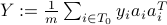 , where
  is an index set accounting for possible data truncation. As asserted in TWF paper, each summand
  follows a heavy-tail probability density function lacking a moment generating function. This causes major performance degradation especially when the number of measurements is small. Instead of spectral initializations, we shall take another route to bypass this hurdle. To gain intuition for our initialization,
a motivating example is presented first that reveals fundamental characteristics of high-dimensional random vectors.
follows a heavy-tail probability density function lacking a moment generating function. This causes major performance degradation especially when the number of measurements is small. Instead of spectral initializations, we shall take another route to bypass this hurdle. To gain intuition for our initialization,
a motivating example is presented first that reveals fundamental characteristics of high-dimensional random vectors.
 |
A curious experiment: Fixing any nonzero vector 
where |
 , generate data
  using i.i.d.
  ,
,  . Then evaluate the following squared normalized inner-product
  is the angle between vectors
  and
and  in an ascending fashion, and collectively
denote them as
in an ascending fashion, and collectively
denote them as ![{xi}:=[cos^2theta_{[m]}~cdots~cos^2theta_{[1]}]^T](eqs/7148505495767972956-130.png) with
with
![cos^2theta_{[1]} %gecos^2theta_{[2]} gecdotsgecos^2theta_{[m]}](eqs/1226858015667637714-130.png) . Figure ref{fig:inner} plots the ordered entries in
. Figure ref{fig:inner} plots the ordered entries in  for
for  varying by
  from
from  %
% ,
,  ,
,  ,
,  , and
, and  with
with  . Observe that almost all
 vectors have a squared normalized inner-product with
  , while half of the inner-products are less than
  , which implies that
 This example corroborates the folklore that random vectors in high-dimensional spaces are almost always nearly orthogonal to each other.
This inspired us to pursue an orthogonality-promoting initialization method. Our key idea is to approximate  by a vector that is most orthogonal to a subset of vectors
  , where
  is an index set with cardinality
  that includes indices of the smallest
squared normalized
inner-products
that includes indices of the smallest
squared normalized
inner-products  .
.
Truncated amplitude based gradient iterations
Precisely, if  and lie in different sides of the hyperplane
  , then the sign of
  will be different than that of
  ; that is,
  . Specifically, one can re-write the
  -th generalized gradient component as

where  .
Intuitively, the SLLN asserts that averaging the first term
.
Intuitively, the SLLN asserts that averaging the first term  over
over  instances approaches
  , which qualifies it as a desirable search direction. However,
certain generalized gradient entries involve erroneously estimated signs of ; hence, nonzero
, which qualifies it as a desirable search direction. However,
certain generalized gradient entries involve erroneously estimated signs of ; hence, nonzero  terms exert a negative influence on the search direction by dragging the iterate away from , and they typically have sizable magnitudes.
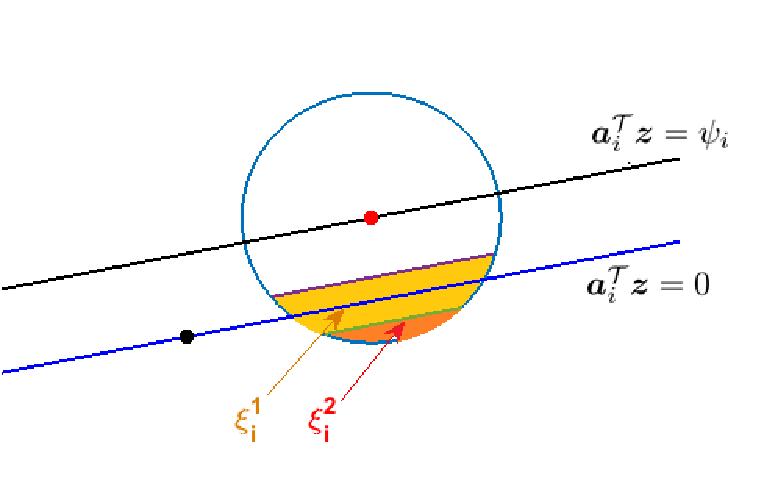 |
The geometric understanding of the proposed truncation rule on the |
 , where the red dot denotes the solution
  and
and  ) passing through points
  and
and  , respectively, are shown.
Nevertheless, it is difficult or even impossible to check whether the sign of equals that of . Fortunately, as demonstrated in Fig. ref{fig:truncation},
most spurious generalized
gradient components (those corrupted by nonzero terms) hover around the watershed hyperplane  . For this reason, TAF includes only those components
having sufficiently away from its watershed, i.e.,
vspace{-.em}
. For this reason, TAF includes only those components
having sufficiently away from its watershed, i.e.,
vspace{-.em}
for an appropriately selected threshold  . To be more specific, the light yellow color-coded area denoted by
  in Figure above
signifies the truncation region of
in Figure above
signifies the truncation region of  , i.e.,
if
, i.e.,
if  obeying the condition above, the corresponding generalized gradient component
  will be thrown out. However, the truncation rule may mis-reject the ‘good’ gradients if lies in the upper part of
  ; and ‘bad’ gradients may be missed as well if belongs to the spherical cap
  .
Fortunately,
the probabilities of the miss and the mis-rejection are provably very small, hence precluding a noticeable influence on the descent direction. Although not perfect, it turns out that
such a regularization rule succeeds in detecting and eliminating most corrupted generalized gradient components and hence maintaining a well-behaved search direction.
.
Fortunately,
the probabilities of the miss and the mis-rejection are provably very small, hence precluding a noticeable influence on the descent direction. Although not perfect, it turns out that
such a regularization rule succeeds in detecting and eliminating most corrupted generalized gradient components and hence maintaining a well-behaved search direction.
 |
 |
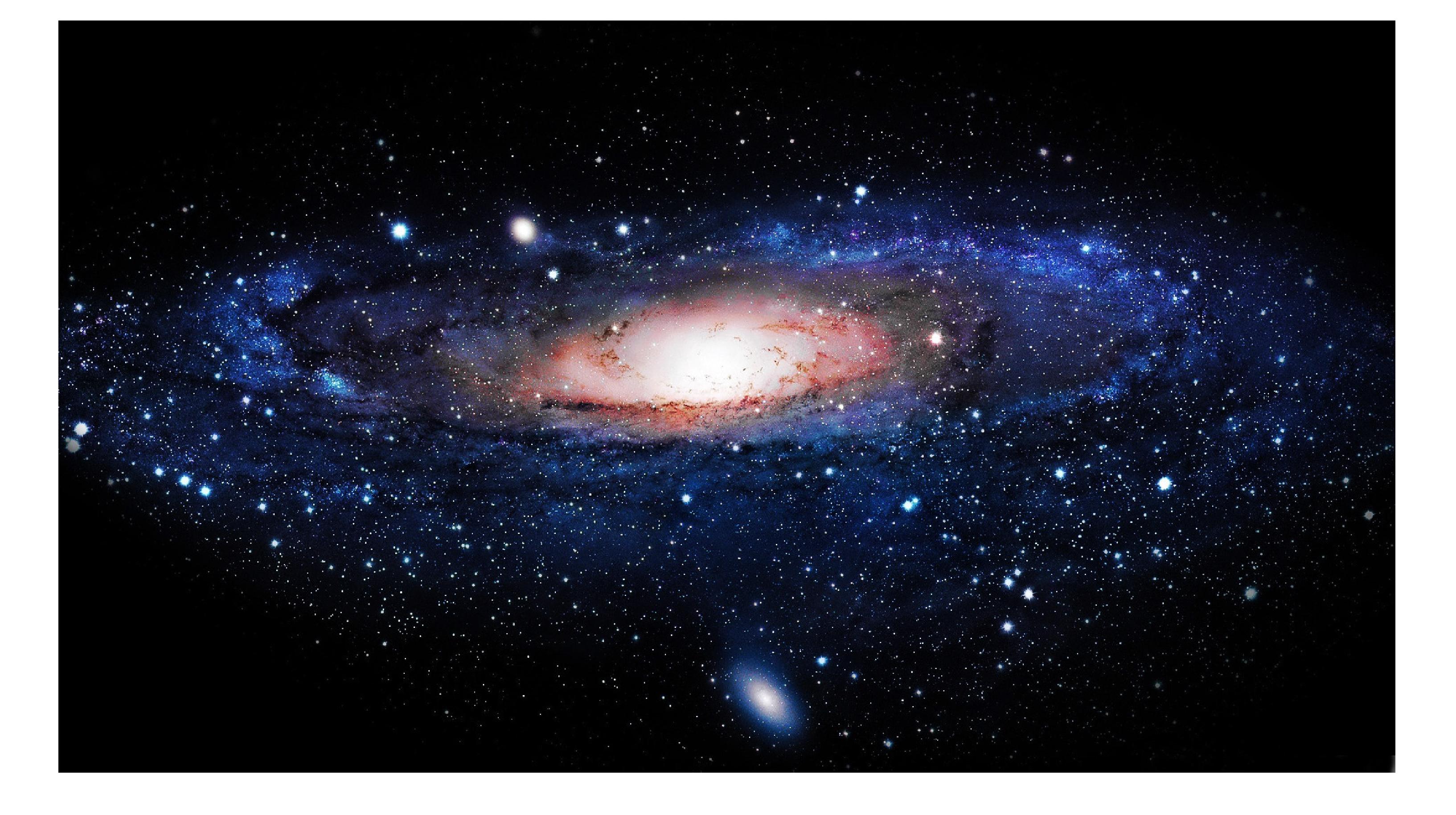 |
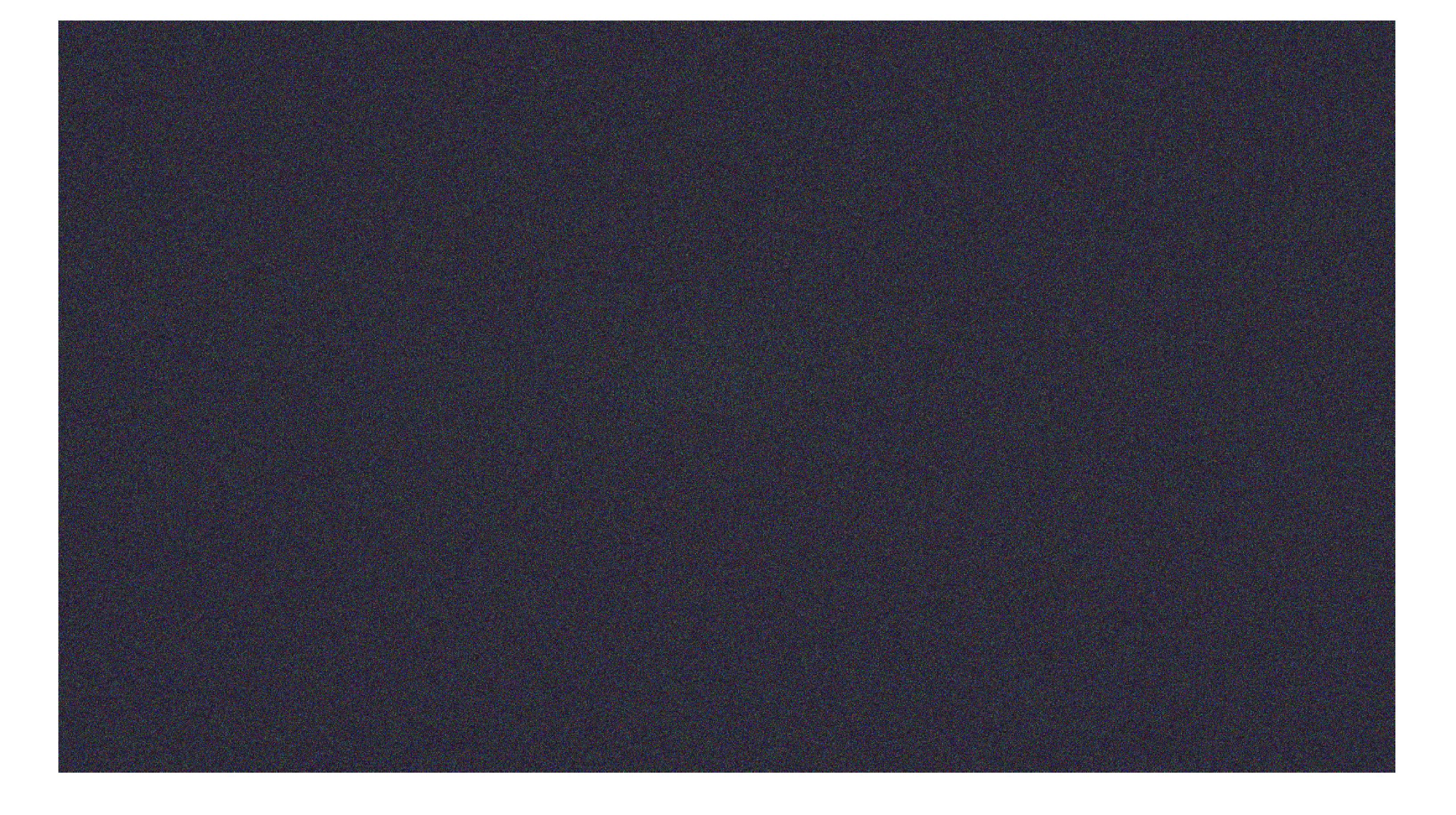
The recovered Milky Way Galaxy images after i) truncated spectral initialization (top); ii) orthogonality-promoting initialization (middle); and iii)  TAF gradient iterations refining the orthogonality-promoting initialization (bottom), where
  masks were employed in our experiment. Specifically, the algorithm was run independently on each of the three bands. A number of power iterations were used to obtain an initialization, which was refined by gradient-type iterations. The relative errors after our orthogonality-promoting initialization and after TAF iterations are
  and
and  , respectively. In sharp contrast, TWF returns images of corresponding relative errors
  and
and  , which are far away from the ground truth.